3.1 Stochastic Properties of Random Matrix Factors

In this series of posts, we will be considering the stochastic properties of factors of random matrices. At first, we look at the simple case of Cholesky decomposition of Wishart matrices. More below.

Let $H$ be a matrix whose elements are random variables, each with a given distribution. Now assume that we factorize $H$ using one of the matrix factorization techniques such as QR, Eigenvalue, or Cholesky decomposition. The elements of the matrix factor are also random variables… but what are their distributions?

This is exactly what we hope to answer.

First and the obvious reason to find the distributions is to understand the characteristics of the matrix factor. For example, in a wireless communication MIMO channel, which is a zero-mean Gaussian random matrix, it helps us understand the stochastic properties of a ”partial” or ”inverse” channel.

The second reason is to speed up simulations. If we have a simulation that requires a random matrix factor which is computed numerically, the simulation may be sped up by generating the elements of the matrix factor directly with the given distributions.

Now we look at the stochastic properties of Cholesky decomposition of Wishart matrices.

Let $G\in {ℂ}^{n\times n}$ be a complex-valued matrix whose elements are Gaussian random variables i.e. $𝒩(0,1)$. Let $H=G^{H}G$. $H$ (Wishart matrix) is now a Hermitian symmetric complex-valued matrix.

It is well known that the Cholesky decomposition of $H$ is the upper triangular matrix from the QR decomposition of $G$, i.e. $H=R^{H}R$ where $G=QR$ for a Unitary matrix $Q$ and an upper triangular matrix with positive diagonal elements $R$.

Therefore, the distribution of $R$ is straightforward from [6] and is given as follows:

where $𝒩$ denotes Gaussian distribution and ${\chi }_k$ the Chi distribution with $k$ degrees of freedom.

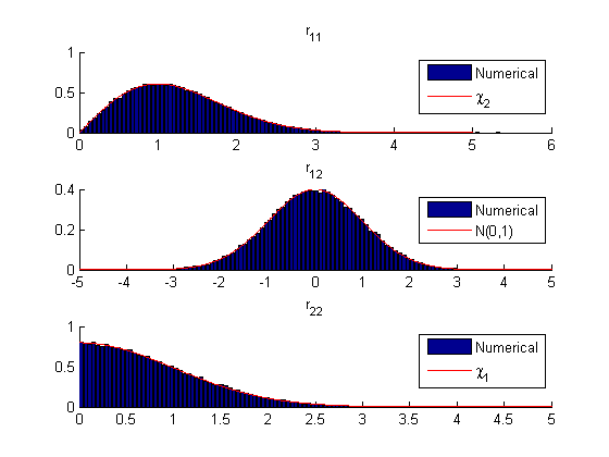
Stochastic properties of the matrix factors may also be verified numerically. Let $G\in {ℝ}^{2\times 2}$ be a real-valued matrix with elements distributed according to standard Gaussian distribution, i.e. $g_{ij}$’s are $𝒩(0,1)$. $G\rightsquigarrow R$ given by:

Figure below illustrates the distributions of elements of $R$ computed numerically using MATLAB. Normalized numerical quantities obtained over 100000 trials are plotted in the blue bar graph and the theoretical expectation is plotted in red. Numerical results closely match the theoretical expectation.

In the next blog posts on this topic, I hope to be able to provide more examples for stochastic properties of matrix factors especially the ones we come across in wireless communication.

In the second on the series of posts on stochastic properties of factors of random matrices, we look at a yet another simple case involving norm square of elements of QR decomposition of a scaled Rayleigh matrices. More below.

In applications such as Non-Orthogonal Multiple Access (NOMA), the so-called ”path loss” plays an important role whereby a channel matrix $𝐇$ at a receiver is better modelled as a scaled Rayleigh matrix given by

$$𝐇=\frac{1}{\sqrt{L}}𝐆$$

where $L>0$ is the path-loss factor and $𝐆$ the conventional Rayleigh matrix with real and imaginary parts of the elements each $𝒩(0,1)$.

Let (by QR decomposition) $𝐇=\mathrm{𝐐𝐑}$ where $𝐐\in {ℂ}^{M\times M}$ is a Unitary matrix, and $𝐑\in {ℂ}^{M\times N}$ is upper triangular. The distribution of the norm square of elements, ${|{[𝐑]}_{ij}|}^2$, of $𝐑$ is given by

where $i=1,2,\mathrm{\cdots },M$, $j=1,2,\mathrm{\cdots },N$, and $\mathrm{\Gamma }(k,\theta )$ denotes the Gamma distribution with probability density function

$$f(x;k,\theta )=\frac{1}{\mathrm{\Gamma }(k){\theta }^k}{x}^{(k-1)}{e}^{-\frac{x}{\theta }}$$

where $\mathrm{\Gamma }(k)$ is the complete Gamma function.

The stochastic properties of the diagonal elements of $𝐑$ are interesting as they can be used to derive insights, amongst others, about mutual information of ”layers” (i.e. parallel streams of information, one per row) or the determinant of the covariance matrix of $𝐇$.

Figure below illustrates the distributions of elements of $𝐑$ for $M=4,N=2$ computed numerically using MATLAB. Normalized numerical quantities obtained over 100000 trials are plotted in the blue bar graph and the theoretical expectation is plotted in red. Numerical results closely match the theoretical expectation.

ARK

In this third post continuing QR and related Cholesky matrix decomposition techniques, we look at the probability density function (PDF) of a diagonal element of the QR decomposition of a complex-valued random matrix with circular Gaussian i.i.d elements.

Let $𝐇$ denote an $N\times N$ matrix with circular Gaussian independent and identically distributed (i.i.d) elements with zero mean and variance two i.e. $𝒞𝒩(0,2)$. Furthermore let $𝐑$ denote the upper-triangular matrix obtained after QR decomposition ($𝐇=\mathrm{𝐐𝐑}$) such that the diagonal elements of $𝐑$ are non-negative. It is well-known that such a QR decomposition (QRP or QR with positive diagonal elements) of a matrix is unique. In case a QR decomposition algorithm results in negative diagonal elements, non-negativity may be arranged by multiplying those rows of $𝐑$ and the corresponding columns of $𝐐$ by -1.

It is well known that the diagonal elements of $𝐑$ follow the distribution:

where ${\chi }_k$ denotes a Chi-distributed random variable with $k$ degrees of freedom.

From the above, it follows that the distribution of a diagonal element $r$ of the matrix $𝐑$ may be given as the (equal) weighted sum of the pdfs of the diagonal elements as

$$f_r(x)=\frac{1}{N}\sum _{n=1}^N\frac{2^n}{\mathrm{\Gamma }(n)}{x}^{n-1}{e}^{-\frac{x}{2}},$$

where $\mathrm{\Gamma }(n)$ is the Gamma function.

The following graph shows the results of a MATLAB simulation for $N=4$ over 100000 iterations where the diagonal values of $𝐑$ were collected. The blue graph shows the histogram of the diagonal values. The red graph shows the pdf as obtained using the equation above. We notice that the two correspond well.

ARK